Abstract
Some animals hunt other animals to feed themselves; these animals are called predators. Animals who are hunted and eaten are known as prey. What do you think would happen if a predator were introduced to an ecosystem where the prey previously lived without fear of being hunted? Would the new predator eat all the prey animals until they go extinct? Actually, the relationship between predator and prey is far more interesting than this. In this article, we show what the predator-prey relationship looks like over time and explain how scientists can make predictions about future population levels, all using basic mathematics like addition, subtraction, and multiplication.
Why Do We Study Animal Populations?
Scientists need to collect information so they can understand how to protect the environment and the animals who live there. Scientists sometimes use mathematics to test theories they have about the animals or even to try to predict the future! This is called mathematical modelling. Modelling the relationship between predators and prey helps scientists understand how their populations change over time, and it can let scientists know when an animal could be at risk of extinction. To make a successful mathematical model, we need to collect data from the environment. In this paper we will show how some basic mathematics, like addition, subtraction, and multiplication, can be used to model the predator-prey relationships seen in the wild.
First, We Need Data!
Good models start with good data. To model a predator-prey relationship, we will use population data (records of how many animals there are) collected by a company that hunted both the predators and prey for their fur in the nineteenth and twentieth centuries. The Hudson Bay Company made yearly records of the numbers of snow lynx and snowshoe hare pelts they collected. Figure 1 shows the company’s data for the number of hare and lynx pelts. The number of hare or lynx pelts collected tells us about the levels of each animals’ population and can give us a reasonable picture of the predator-prey relationship. The data show that in some years, like 1927, there were more lynxes (predators) but fewer hares (prey), while in other years, like 1932, there were more hares but fewer lynxes.
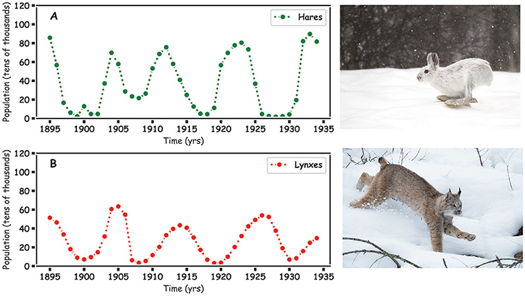
- Figure 1 - (A) The number of hare pelts collected (in tens of thousands) over time.
- (B) The number of lynx pelts collected (in tens of thousands) over time, inferred from Hudson Bay Company data from 1895 to 19351.
What Does The Hudson Bay Data Tell Us?
The rise and fall in the recorded hare and lynx populations over time suggests that there is a relationship between the two animals, which makes sense as we know that lynxes eat hares. In Figure 1, can you see that the populations of lynxes and hares fall and rise at around the same time? When there are more lynxes they eat more hares, which decreases the hare population. When the hare population is low, this means less food for the lynxes and results in a decrease in the lynx population. When the lynx population decreases, the hare population increases again, and the up-down cycle continues. If the predator and prey populations are balanced, they will go up and down over time, chasing each other in the circle of life. The question a mathematician asks is, “Can I explain this using addition, subtraction, and multiplication; and can I predict the future populations”
Explaining The Relationship With Mathematical Models
Mathematicians use differential equations and data to describe what they see in the world. The predator-prey relationship was first described using differential equations by two scientists named Lotka [1] and Volterra [2]. They wanted to use mathematics to explain the rise and fall observed in the general predator-prey relationship.
The equations can sometimes look very complicated, but all they are is a way to describe how and why populations change. A famous mathematician named Leonhard Euler (1707–1783) showed that differential equations could just be written as pluses and minuses, with a bit of multiplication. Differential equations can be used to model the populations of lynxes (predators) and hares (prey) using the data from the Hudson Bay Company. We fit the original data using mathematical methods [3], to estimate the values for the growth rate (rgrowth),death rate (rdeath),eaten rate (reaten), and food rate (rfood), which we will use to predict the hare and lynx populations.
Modelling the Snowshoe Hare Population
When developing an equation, a mathematician thinks about the world. Now, let us think about what is happening to the hare population over time. If there were no lynxes, then the hare population in the future, HF, would be equal to the current hare population, HC, plus births and minus deaths. We call this the growth rate, rgrowth. The number of births and deaths will depend on the how many hares are alive now, so we multiply rgrowth by HC (Figure 2A).
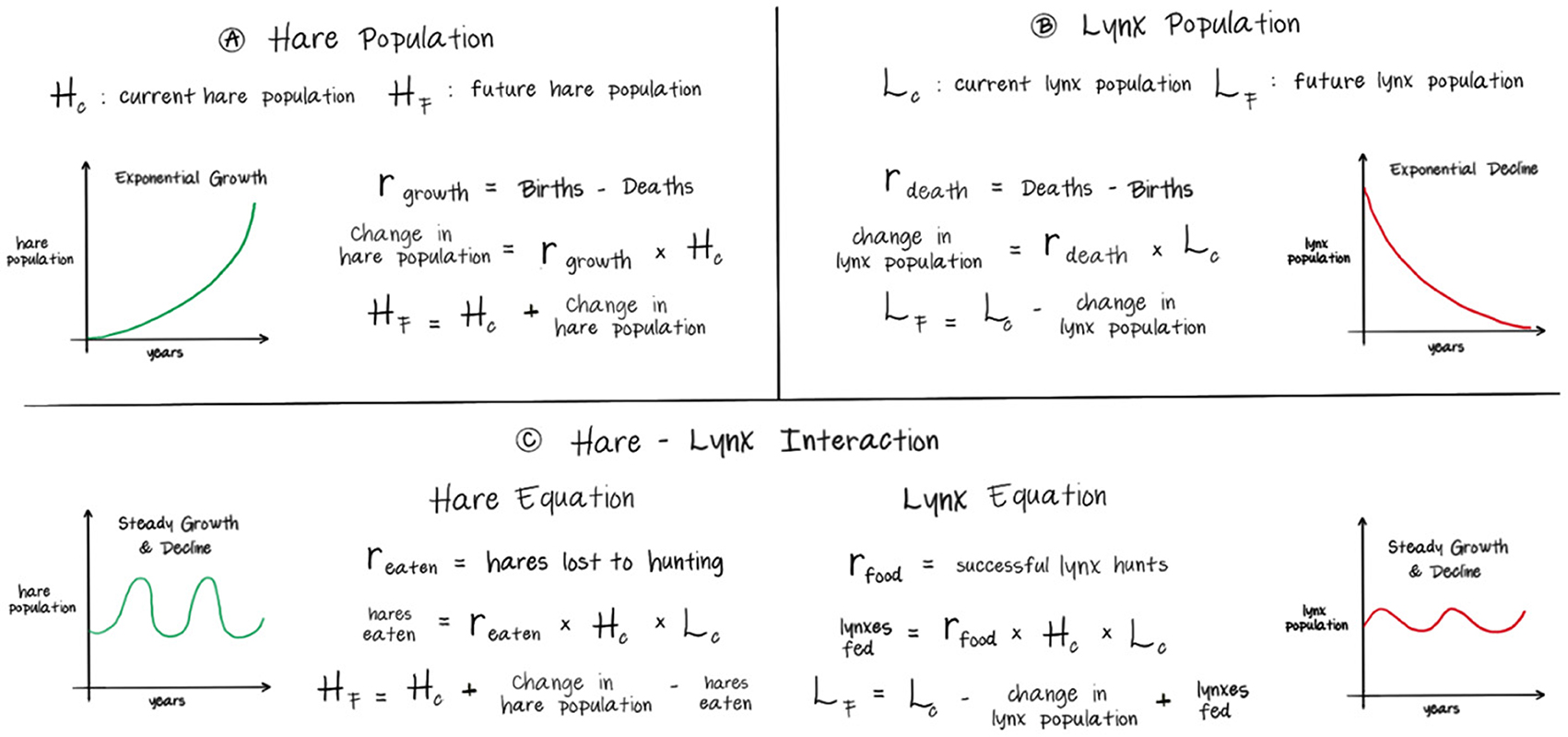
- Figure 2 - (A) The equations used to predict the future hare population if there were no lynxes, which results in exponential growth.
- (B) The equations used to predict the future lynx population if there were no hares, resulting in exponential decline. (C) The equations for the hare and lynx populations when the populations are interacting with each other. This results in fluctuating population levels for both hares and lynxes.
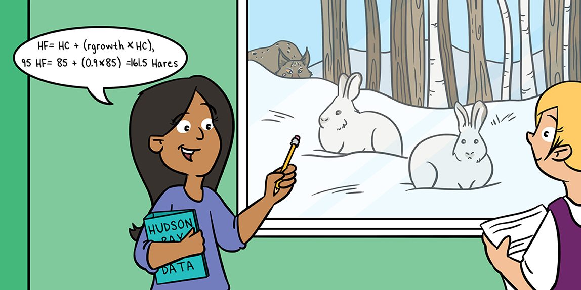
Let us use the Hudson Bay data to put numbers into the equation. when the data starts in 1895, the hare population is 85, so we will let HC = 85 hares. The growth rate for the hare population is rgrowth = 0.9 in a year. Since rgrowth is positive, we expect the future population to grow. This gives the future hare population HF in 1896:
HF = HC + (rgrowth × HC), HF = 85 + (0.9 × 85) =161.5.
We predict that the future hare population will be 161.5 hares. If the population keeps growing like, this the entire world will be covered in hares, which is called exponential growth (Figure 2A).
Modelling the Snow Lynx Population
Let us next consider what is happening to the lynx population over time. If there are no hares, the lynxes would have no food, so the lynx population would go down. To model this, we use subtraction. The future number of lynxes (LF) is equal to the current number of lynxes (LC) minus the death rate, rdeath, times the current number of lynxes (Figure 2B).
The lynx population in 1895 is 51, and by fitting the data we set the death rate to rdeath = 0.25. Now the equation gives:
LF = LC-(rdeath × LC),
LF = 51–(0.25 × 51) = 38.25.
Our calculation predicts the future lynx population in 1896 to be 38.25 lynxes. This is known as exponential decline and, if it keeps happening, there will be no lynxes (Figure 2B).
Modelling the Hare and Lynx Interaction
On their own, the hare population increases, and the lynx population decreases. What do we know about how these populations interact with each other? Lynxes eat hares and so decrease the hare population; therefore, we use subtraction to model this. We need a term for the eat rate, reaten, which depends on both the current lynx and hare populations available to both eat and be eaten. So, we multiply reaten by LC and HC.
By the same logic, the hares are a food source for the lynxes, so we use addition in the lynx equation and multiply the current hare population by the current lynx population times a food rate, rfood (Figure 2C).
The values of HC = 85 hares, rgrowth = 0.9, LC = 51 lynxes, and the rdeath = 0.25 remain the same. From the data, we get an eat rate of reaten = 0.024 and a food rate of rfood = 0.005. Putting these numbers into the equation for predicting the future number of hares gives:
HF = HC + (rgrowth × HC) – (reaten × LC × HC),
HF = 85 + (0.9 × 85) – (0.024 × 85 × 51) = 59.24,
and the equation for predicting the future number of lynxes now gives:
LF = LC-(rdeath × LC) + (rfood × LC × HC),
LF = 51–(0.25 × 51) + (0.005 × 51 × 85) = 59.925.
Our model (both equations above) predicts a decrease in the hare population and an increase in the lynx population in 1896, as shown in Figure 3 by the green and red arrows.
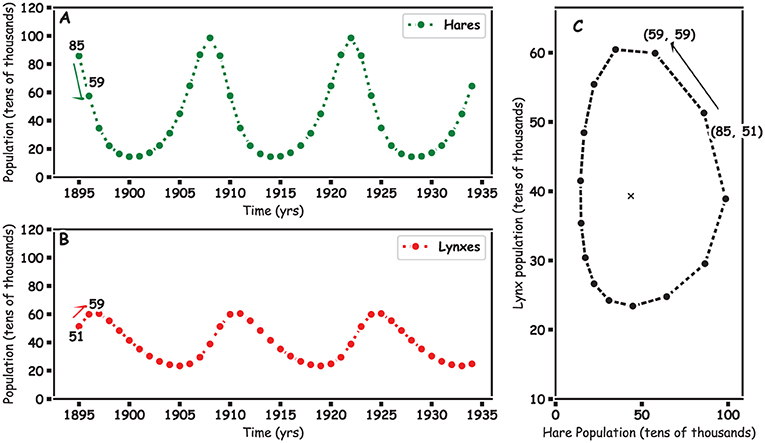
- Figure 3 - Hare and lynx populations modelled using the equations and the Hudson-Bay Company data from 1895 to 1935.
- (A) The modelled hare population. (B) The modelled lynx population. These two plots show the rise and fall that we saw in the real data in Figure 1. (C) How the lynx population changes for different hare populations. The x is the mean lynx and hare population, which the two populations orbit. The arrows and numbers indicate the calculations in the text, from 1895 to 18962.
To predict how the populations would change in the following year, 1897, we would plug our HF and LF values into HC and LC in the new equations. Each time we do this we get new values, and each value is a point for our graphs in Figure 3.
Visualising The Predator Prey-Relationship
Using the equations from above and some computer code [4], we simulate both the hare and lynx populations and make our own data showing how the predator-prey relationship evolves over time (Figure 3).
Another way to show how two species are linked is to plot how the hare population (x-axis) and lynx population (y-axis) change in relation to each other (Figure 3C). The x in the middle shows the average hare (39) and average lynx (45) populations, known as the equilibrium point. The lynx and hare populations circle around this average as the populations rise and fall, plotting the circle of life. It looks a bit like the orbit of the earth around the sun. The populations go around and around, which represents their ups and downs over time. In a balanced ecosystem, like the one modelled here, the orbit stays stable; but if it starts spiralling in or out, this could be an early sign of change.
One such change occurred in 1995, when wolves were re-introduced to Yellowstone Park. This lead to some surprising results for the surrounding ecosystem3. Based on these amazing observations and mathematics similar to what we have shown here, Goodman and colleagues developed a computer game to build a balanced eco-system4.
Models Are Not Exact
When mathematicians try to describe something complicated, they simplify things. The equations we have shown must simplify things, too. The simplifications mean that the predictions and simulations do not perfectly follow the original data. Here is some information we left out of our model:
- There is more than one predator of the snowshoe hare.
- Snow lynxes hunt more than just snowshoe hares; they can also eat fish and squirrels.
- In our model, the snowshoe hares do not run out of food, which is not true in winter.
- What about human fur hunters who hunt both lynxes and hares?
To make the equations work for all these other situations, we would have to include extra equations and more pluses and minuses. If we have all the data, we could perfectly model the future. Even with these simplifications, the mathematics still does a good job modelling the hare and lynx populations.
How Else Can This Model Be Used?
If you change the words “snow lynx” to “shark” and “snowshoe hare” to “fish” in this model, the mathematics will still work, with the right data [2]. You could even use the same equations and change the word “lynx” to “zombie” and “hare” to “human”! The predator-prey relationship can be expanded further outside of animal populations and can be used to model how companies interact, how chemical reactions occur, and how viruses spread. You can read more about the mathematics of viruses in another Frontiers for Young Minds paper by clicking here [5].
Summary
To develop models of the real world, mathematicians need to start with good data. This means it is vital for scientists, conservationists—and even fur hunters!—to collect information from the environment around them. Using data, we can spot patterns in relationships and then use mathematics to recreate these patterns and predict future data that can represent and predict the future of those relationships. These predictions can help us maintain balanced ecosystems. Hopefully, from this article, you can see how all it takes is the basic mathematics of adding, subtracting, and multiplying—and a bit of clever thinking—to model and predict the populations of a predator, its prey, and much more.
Glossary
Differential Equations: ↑ Equations that describe how populations change over time, or describe many other processes, including how a helicopter flies, how planets orbit a star, or how blood flows in our veins.
Estimate: ↑ A value that is close enough to the exact answer, usually created based on some knowledge you have of the system or by preforming a calculation.
Growth Rate: ↑ The growth rate is the increase of the hare population if they had no predators. It can be estimated from the data using the number of births minus deaths.
Death Rate: ↑ The death rate is the decrease of the lynx population over time if they had no food. This is the number of deaths minus births.
Eat Rate: ↑ The eat rate is the number of hares hunted and eaten by the lynx.
Food Rate: ↑ The food rate is the number of hares the lynx need to eat to survive.
Exponential Growth: ↑ Steady and rapid growth.
Equilibrium Point: ↑ The balance point in the two populations. When a system is in equilibrium, we say it is stable.
Conflict of Interest
The authors declare that the research was conducted in the absence of any commercial or financial relationships that could be construed as a potential conflict of interest.
Acknowledgments
This work was supported by Irish Research Council funding (GOIPG/2020/943).
Footnotes
1. ↑Link to animated version of the figure here.
2. ↑Link to animated version of the figure here.
3. ↑Watch: Sustainable Human 2014.
4. ↑Play here: https://ecobuildergame.org.
References
[1] ↑ Lotka, A. J. 1920. Analytical note on certain rhythmic relations in organic systems. Proc Natl Acad Sci USA. 6:410–5.
[2] ↑ Volterra, V. 1926. Fluctuations in the abundance of a species considered mathematically. Nature. 118:558–60.
[3] ↑ de Silva, B. M., Champion, K., Quade, M., Loiseau, J. C., Kutz, J. N., and Brunton, S. L. 2020. PySINDy: a python package for the sparse identification of nonlinear dynamics from data. arXiv Preprint arXiv:2004.08424.
[4] ↑ Butler, J. S., and Brady, R. M. 2020. Predator Prey Code for Young-Minds. GitHub. Available online at: https://github.com/john-s-butler-dit/Predator-Prey-for-Young-Minds
[5] ↑ Brooks, H. Z., Kanjanasaratool, U., Kureh, Y. H., and Mason. P. 2021. Disease detectives: using mathematics to forecast the spread of infectious diseases. Front Young Minds. 9:577741. doi: 10.3389/frym.2020.577741