
Abstract
Many things in our lives are designed to solve problems. Whether it is an app on our cellphones, the construction of a new building, or the development of a new drug, solving problems is a big motivator. Did you know that there is a fascinating type of mathematics behind many of the complex problems we face in our daily lives? This mathematics is called computational complexity theory, and it is a field of computer science. This is an active, constantly developing field that is attracting many talented young people—like you! In this article, we will describe computational complexity theory and the kinds of problems it is designed to help with. We hope that by the time you finish reading this article, you will be convinced that computational complexity theory is one of the most exciting fields of science.
Noa Segev is a scientific writer and project coordinator at Frontiers for Young Minds. She has a B.Sc. in physics and an M.E. in renewable energy engineering.
Prof. Avi Wigderson won the 2021 Abel Prize, jointly with László Lovász, for their foundational contributions to theoretical computer science and discrete mathematics, and their leading role in shaping them into central fields of modern mathematics.
Computational Complexity Theory
When you think about the word “computation,” you probably think about numbers—maybe about the processes of addition and multiplication that you learned in your school math classes. Although those math operations are indeed computations, the term computation is actually much broader and includes many of the challenges we face in daily life, like the need to compute how to get from one place to another as quickly as possible, or how to keep sensitive information safe using encryption. The field of computer science that deals with many of the complex problems we face in our everyday lives is called computational complexity theory. Each computational complexity problem has an input and one or a bunch of valid solutions—not only one. For example, think about a navigation app like google maps. This app must solve the computation problem of how to get from point A to point B the fastest way possible. There could be a few different routes that take you from point A to point B in the same amount of time, and therefore this computation theory has a few equivalent solutions. The inputs in this case are the start and end points (A and B), and the solutions (also called the output) of the computations are all the possible routes you could take to get from point A to point B as quickly as possible.
The solution of a computational problem requires two stages (Figure 1). The first stage is defining the function connecting the input and output. Once a function is given, the second stage involves finding an efficient way to solve the problem, to estimate the solution, or to prove that the problem is hard and cannot be solved in a reasonable time—that is the job of computer scientists who deal with computational complexity theory.
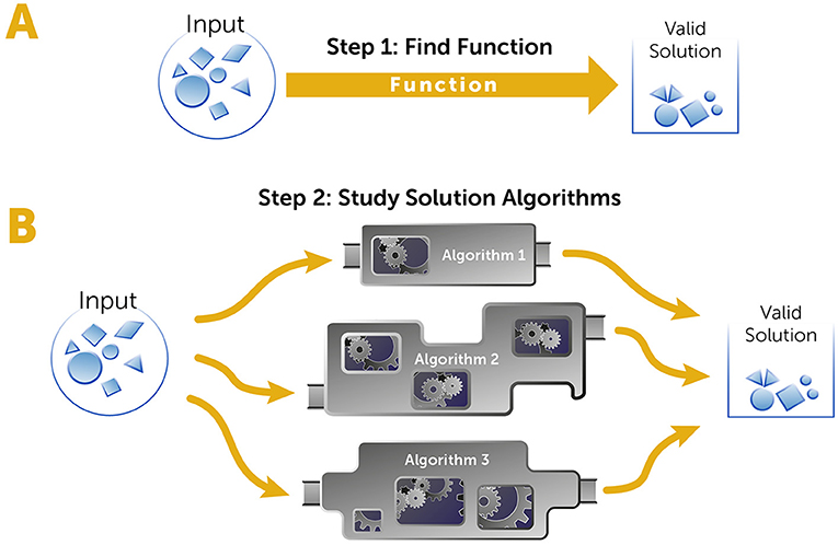
- Figure 1 - A computational complexity problem.
- Computational complexity problems have a collection of valid solutions—not just one—for every input. Solving these problems requires two stages. (A) In the first stage, we must define the problem clearly or, in other words, describe the function connecting the input to the collection of valid solutions. This is usually the work of physicists, biologists, chemists, economists, or engineers. (B) In the second stage we look for algorithms—the series of operations that can solve the problem most efficiently. This is the stage is generally performed by computer scientists.
An important problem from biology—called the protein folding problem—can be used to demonstrate the stages of solving a computational problem. As you may know, our bodies contain tiny biological machines called proteins that perform many of our vital functions. Proteins are made of chains of building blocks called amino acids (like a bunch of beads on a string), and after they are made, these chains fold into complex, three-dimensional structures (see Figure 1 in this article). Proteins only function properly if they fold into the correct three-dimensional shapes. Scientists still do not know the exact physical and chemical laws that make proteins fold in the very specific ways that they do, out of all the millions of possible ways they could fold. This protein folding problem is a computational problem—for every specific chain of amino acids (the input), there is one solution of a specific three-dimensional that allows the protein to function. Scientists have created several models to try to describe how the amino acid sequence of a protein determines its final three-dimensional structure. One model uses the idea that the final structure of the protein is the one that needs the least energy to hold the shape. This can be calculated by adding up the attraction or repulsion forces of each pair of atoms that make up the protein [1]. Defining a model is the first stage in the solution process.
The next stage is the computational stage, which tries to determine how hard it is to calculate the solution to the problem, and to figure out the most efficient way to compute the solution—which in this case is to find the final three-dimensional structure of the protein. For example, if the protein only has a small number of atoms, it is easy to compute all the forces acting between every pair of atoms and add them up to figure out the three-dimensional structure that requires the least energy. But, if the protein is composed of many atoms (as most proteins are), it is much harder and sometimes even impossible to compute the exact folding that results in the minimal energy, even if we use very powerful computers. Maybe, in these cases, there is a better calculation that would allow a solution to be found? That is the kind of challenge that computational complexity theory deals with.
Computational complexity theory can deal with many practical questions that are related to our daily lives. In addition to helping us build models of systems we want to understand, like the protein folding problem, computational complexity theory can also be used to figure out what kinds of problems can and cannot be solved, to determine how efficient computations are at solving problems, and to develop practical tools for solving problems. This may sound complicated, but you will see that it is a beautiful and fascinating field of research.
Algorithms and Efficiency
One of the most important problems in computational complexity theory deals with the efficiency of computations [2]. Every computation is defined by a collection of operations that are performed on the input to get to the result. This collection of operations is called an algorithm. We all use algorithms in our daily lives. For example, we all learn to add numbers in school. You may have learned to add according to the algorithm shown in Figure 2A. Any two numbers can be added, which means there are an unlimited number of inputs into the addition algorithm. Inputs could be one digit, a million digits, or a billion digits, for example. The most efficient computations are like adding numbers: the number of operations required in the algorithm is proportional to the length of the input numbers. This means that, using the algorithm described in Figure 2A, if we had to add numbers that were twice as long as the numbers shown, we would have to perform twice as many operations to get the final result.
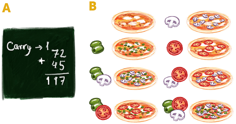
- Figure 2 - Computational complexity.
- (A) An easy algorithm for adding numbers. The number of required operations is proportional to the length of numbers being added. If we increase the numbers from 2 to 4 digits, then twice as many operations are needed. (B) An algorithm to compute all the possible combinations of pizza toppings is exponential. The number of operations is proportional to 2 to the power of the input’s length. If there are three possible toppings (inputs), the number of required operations is 23, meaning that there are eight possible topping combinations. For exponential algorithms, the number of required operations grows very quickly as the input length increases, so the computation times needed for these algorithms are only reasonable for small inputs.
But let us think about a slightly more difficult problem: multiplying numbers. In school, you were probably taught an algorithm for this, too. If you use the algorithm shown in this video, if you want to multiply numbers that are twice as long, the number of operations you must perform will be 4-fold greater. For example, if we multiply two two-digit numbers, we perform four multiplication operations and a few more addition operations. However, if the numbers have ten digits, we must perform 100 multiplication operations! If we use the algorithm shown for addition, only 10 operations would be required for 10-digit numbers. If the numbers have 100 digits, we need to perform about 10,000 operations for multiplication as opposed to about 100 operations for addition. So, in the case of multiplication, the number of operations is proportional to the square of the numbers’ lengths.
The efficiency of computations is very important because it defines which problems we can solve within a reasonable time and which we cannot, and the cost (in effort and time) required for each computation. There are many problems we must solve quickly so that the answer can be available to us almost immediately (for example, like Waze, which should instantly tell us which route to choose), and there are some problems we want to solve within a reasonable time (not necessarily immediately) to find answers to important questions in science or engineering, for instance. As you saw in the addition and multiplication examples, the difference between the efficiency of an algorithm that is proportional to the length of the input and one that is proportional to the squared length of the input is large. Let us now think about a case in which the algorithm is proportional not to the squared length of the input, but to an even higher exponent—maybe to the fifth or sixth power. Or we could think about a case in which the algorithm’s efficiency is exponential, meaning proportional to two in the power of the input’s length, or even a larger number in the power of the input’s length. These cases require many computations to get to the solution.
Such complex problems do exist in our daily lives. To demonstrate the meaning of an exponential function, here is a tasty example—think about your favorite pizza. Let us say that the pizza restaurant had one possible topping—green olives. Then, you could choose between two options: a plain pizza or a pizza with green olives. Now, let us assume that the pizza place also has a corn topping. Then, you could choose between four options: plain, with green olives, with corn, or with green olives and corn. If there were three toppings (for example, mushrooms, olives, and tomatoes) you would have eight possibilities (Figure 2B). So, in this case, there are two to the power of possible topping options (23 = 8). Therefore, the number of options for pizza topping combinations is exponential with respect to the number of toppings, which is basically the input length in the calculation. For larger inputs, like tens or hundreds of pizza toppings, the number of topping combinations quickly becomes enormous.
Exponential Algorithms
The same exponential type of growth applies also for exponential algorithms. Now, instead of the length of input growing exponentially (like we saw with the number of possible pizza toppings), it is the number of operations in the algorithm can grow exponentially and is proportional to some number (say two, like in the pizza example) in the power of the input’s length. Since the number of operations a computer can perform is finite—a billion operations per second, say—we can translate the number of operation into the time it takes for computation. For an exponential algorithm and a 20-character-long input, the computation time for such a computer will be only one-millionth of a second. For a 50-character input, the computation will take more than 18 min, and for an 80-character input, it will take more than 3,800 years!
Since there are many computations we would like to be able to perform in a reasonable time, one major question in complexity theory deals with trying to find the most efficient algorithms to perform certain computations. For example, you may have learned a quicker way than the one we described for multiplying two numbers (you can watch an example here). In the same way, it might be possible to find more efficient ways to perform other computations for which we have only inefficient solutions. Researchers studying computational complexity theory search for these efficient algorithms and, to do so, they must also ask themselves how they know when they have found the best, most efficient algorithm. Sometimes they can prove that an algorithm is the best possible one for a particular problem, and other times they try to prove that there is no efficient way to solve a particular problem for every input, meaning that the problem is inherently hard.
Easy and Hard Problems to Solve
Now let us think about dividing all problems into two groups depending on how difficult it is (i.e., how much time it takes) for a computer to solve them [2]. We will call one group P, for “polynomial”. Problems in P be solved quickly, because the number of computations needed to solve them is equal to the input’s length to some power. For example, when adding numbers according to our algorithm, the number of operations required is a polynomial of the first power with respect to the input’s length. We can think of problems in P as all the problems that humanity can solve or has already solved.
The second group of problems is called NP, for “nondeterministic polynomial”. This is the collection of problems that have not been solved yet, but that humanity would like to solve. Real-life problems in NP include, for example, all the problems that scientists think about, all mathematical proofs that mathematicians are trying to validate, and engineering problems such as planning a bridge that spans a river (Figure 3A).
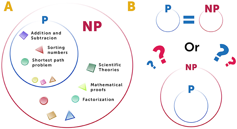
- Figure 3 - Problems in P and NP—are they equal?
- (A) Currently, problems can be divided into two sets. P contains problems that can be solved efficiently and NP contains problems whose solutions can be checked efficiently. (B) A very important question within complexity theory is whether for all problems in NP there is an efficient solution algorithm. This would mean that P and NP are equal. Alternatively, NP could include all problems that are in P but also include additional problems that are not in P, that cannot be solved efficiently.
Sometimes a problem might be difficult to solve, but once a solution is found, checking to see if that solution is correct might be relatively easy. Imagine a strange navigation app that needs to find the longest possible route between two points, instead of the shortest. This is a hard problem—finding the longest possible route between two points is much more complex than finding the shortest route. However, if we were given all the possible routes between two points, it would be easy to check which route is the longest, just by comparing them. In other words, even if the computation of the original problem is complex, checking a suggested solution is easy. As another example, if we try to find all the factors of a very large number (meaning, numbers that can be multiplied together to get that large number) this could be a hard problem. In contrast, if we just need to check whether two numbers are factors of a large number, this is an easy problem—we only need to multiply them together to check if the solution equals that large number.
One of the biggest open questions in computational complexity theory is whether the classes of P and NP problems are equal or whether P is a subgroup of NP (Figure 3B). In other words, if we can easily check whether a given solution to a problem is correct, does this definitely mean there is an algorithm that solves that problem efficiently, even if we have not found it yet? We do have examples of problems in NP for which we have not found efficient solutions—but this does not mean that such algorithms do not exist—maybe we just have not found them. If they do exist and we will be able to find them, this might be humanity’s biggest dream coming true. On the other hand, there are some problems that we hope are too hard to solve (i.e., not in P). For example, the safety of data-encryption systems and other electronic safety system like those used for online shopping are based on extremely complex calculations that we hope are too hard to ever solve efficiently. If someone finds an efficient algorithm to solve these calculations, all of our information-protection systems will break down and the information that is currently safely encrypted will no longer be safe. So, you can see that there are reaching implications to the questions whether P and NP are equal classes of problems.
Recommendations for Young Minds
Our main recommendation is to find out what you love—what your passion is. People do their best and most significant things when they believe in the importance of what they are doing, and often what is important for them is also fun for them. You might have a strong motivation to do things you do not necessarily enjoy all the time (for example, maybe you want to cure cancer but do not enjoy the lab work), but we think this option is not quite as good as finding something you really love.
If you enjoy problem solving, we recommend that you learn as much as possible and try to understand the kinds of problems that you like to face. Once you choose an area, try to be the best you can (Figure 4). An academic career is not for everyone, and some people might have more fun working in industry in companies that try to solve various problems. But if you are interested in an academic career, develop two important characteristics: an unstoppable thirst for knowledge and a love for sharing that knowledge through teaching and guiding students. Patience is also important, along with the ability to handle a competitive environment in a positive way.

- Figure 4 - Recommendations for Young Minds.
- Learn a lot and discover the kinds of intellectual problems you like to face. If these problems are in mathematics, remember that many mysteries you try to crack will include moments of “failure,” in which you will not solve the problem or even know whether you are progressing toward the solution. Remember that these “failures” give you extremely valuable insights and experience that will help you solve other problems in the future.
If you are specifically interested in mathematical research, remember that there are connections between sub-fields that supposedly do not “talk” with each other. These connections are critical, so it is important to have knowledge of as many fields of math as possible. In addition, mathematicians often try to solve problems that no one has solved before, so if you follow that path there is a chance that you will not solve them, either. That means that you might invest a lot of time on things that are ultimately unsuccessful. But if you enjoy the problem-solving process, then even if you have no promise that your solution will work, or even if your progress seems extremely slow, you will still be happy. In other words, good math researchers must love the process of solving problems, independent of how successful the process is. Finally, it is important to remember that researchers are always learning from the ideas that they try, even if they are not successful in solving the problem. The insights they gain in the process stay with them and can help them to solve future problems.
Author’s Note
This article is based on an interview between the two authors. It is written in the artistic expression of NS and is backed up scientifically by AW.
Glossary
Algorithm: ↑ A collection of actions that are performed on the input to get to the computation result in a finite number of steps.
Problems in P: ↑ Computational problems whose solution is easy (polynomial with respect to the inputs’ length).
Problems in NP: ↑ Computational problems for which checking their solution is a problem in P. Such algorithm does not provide the solution but only makes sure that a suggested solution is correct.
Conflict of Interest
NS declared that they were an employee of Frontiers, at the time of submission. This had no impact on the peer review process and the final decision.
The remaining author declares that the research was conducted in the absence of any commercial or financial relationships that could be construed as a potential conflict of interest.
Acknowledgments
We wish to than Alex Bernstein for providing the figures.
References
[1] ↑ Levinthal, C. 1968. Are there pathways for protein folding? J. Chim. Phys. 65:44–5.
[2] ↑ Wigderson, A. 2019. Mathematics and Computation. Princeton, NJ: Princeton University Press.