Abstract
Suppose that you are going to school and arrive at a bus stop. How long do you have to wait before the next bus arrives? Surprisingly, it is longer—possibly much longer—than what you might guess from looking at a bus schedule. This phenomenon, which is called the waiting-time paradox, has a purely mathematical origin. In this article, we explore the waiting-time paradox, explain why it occurs, and discuss some of its implications (beyond the possibility of being late for school).
How Long Do You Have to Wait for the Next Bus?
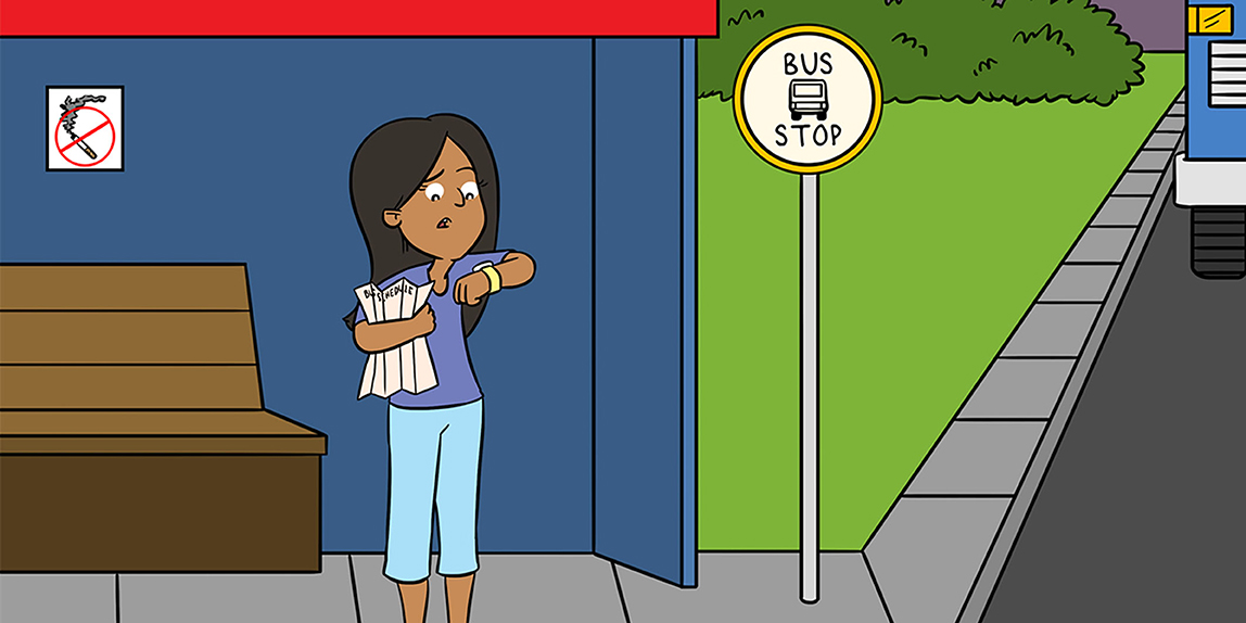
Suppose that you live in a city and take a bus to go to school. Because buses come frequently in your neighborhood, perhaps you do not need to pay close attention to the bus schedule. Maybe you just go to the closest bus stop and ride the next bus (see Figure 1A). However, if you arrive and have no idea when the next bus is coming, how long do you have to wait for the next bus?
- Figure 1 - (A) You arrive at the bus stop to wait for the next bus.
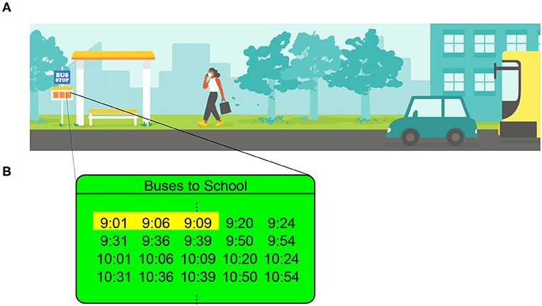
- (B) You look at the schedule and see that there are 10 buses each hour. This is an average of one bus every 6 minutes. The first three buses after 9:00 are scheduled to arrive at 9:01, 9:06, and 9:09. We highlight these three times in yellow. The inter-event times—in other words, the times between consecutive buses—are 5 minutes (between the first and second buses) and 3 minutes (between the second and third buses). [Panel A was drawn by Iris Leung.]
Suppose that 10 buses come each hour (see Figure 1B), so one bus comes every 6 minutes on average. If the most recent bus leaves right before you arrive, you may have to wait 5 or 6 minutes for the next bus. If the most recent bus leaves a few minutes before you arrive, maybe the next bus will come in only 1 minute. Or maybe 4 minutes, or perhaps 2 minutes? An educated guess for your “waiting time” is 3 minutes, which is half the time between buses on average. However, this reasoning is incorrect. Typically, you must wait longer than 3 minutes. Your expected waiting time can be even longer than 6 minutes. This phenomenon is called the waiting-time paradox [1, 2]. A paradox is a something that seems like it does not make sense but actually turns out to be correct. Many people think of the waiting-time paradox as a paradox because a typical waiting time at a bus station is longer than half of the average interval of time between buses (which is 3 minutes in the example above). The waiting-time paradox is a mathematical phenomenon and has nothing to do with buses. What is this phenomenon and how does it fool us? Keep reading to find out!
Why Does the Waiting-Time Paradox Occur?
To understand why the waiting-time paradox occurs, consider the bus schedule in Figure 2A. In this schedule, which is simpler than the one in Figure 1, buses arrive at either 4-minute or 12-minute intervals. The original bus schedule in Figure 1B has various irregular-looking numbers, and there are several different intervals between bus arrivals. In general, when a situation looks complicated, it is useful to simplify it before applying mathematical reasoning. People who work with mathematics do this all of the time. The waiting-time paradox also occurs in the simplified bus schedule, and the simplification makes it easier to understand what is going on.
- Figure 2 - Comparison between the naive guess of an average waiting time and the actual average waiting time.
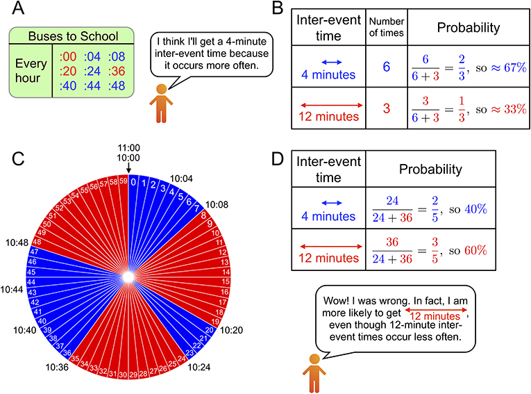
- (A) A simplified bus schedule. (B) Naive guess about the probabilities of getting 4-minute and 12-minute inter-event times. This guess is based on the incorrect idea that a 4-minute inter-event time is more likely than a 12-minute one because it occurs more often. (C) Showing the inter-event times in 1 hour as a pie chart can help us understand why this is not correct. (D) The actual probability of getting a 12-minute inter-event time is larger than the probability of getting a 4-minute one because there are 36 red slices but only 24 blue slides in the pie chart in (C).
A key concept that we need to consider is the inter-event time, which is the time between two consecutive buses. The schedule in Figure 2A indicates that, in each hour, six buses arrive immediately after an inter-event time of 4 minutes (blue) and three buses arrive immediately after an inter-event time of 12 minutes (red). In our scenario, recall that you have arrived at the bus stop without knowing when the next bus will arrive. In the language of probability theory, we say that you arrive at the bus stop at a time that has been chosen uniformly at random. Do you think that you are more likely to have a 4-minute inter-event time or a 12-minute one? If you get a 4-minute inter-event time, you will not wait very long for the next bus. However, if you get a 12-minute one, you may have to wait a long time. As we mentioned above, six inter-event times are 4 minutes long and three inter-event times are 12 minutes long.
Think about it this way: perhaps you are likely to get a 4-minute inter-event time because there are six of them each hour, but 12-minute inter-event times occur only three times each hour. The former occurs with a probability of 6/(6 + 3) = 2/3, which is about 0.67, so this situation occurs about 67% of the time (see Figure 2B). The latter occurs with a probability of 3/(6 + 3) = 1/3, so this situation occurs about 33% of the time. Unfortunately, this is wishful thinking. Arriving at a bus stop uniformly at random is like spinning a wheel with the numbers 0 through 59 on each “slice” of the wheel (so there are 60 slices in total), stopping it with your finger, and looking at the slice that your finger is touching. If your finger points to 33, it means that you arrive at the bus stop at 10:33. In this case, you need to wait 3 minutes for the next bus, which arrives at 10:36. The wheel gives a way to help us understand the notion of “uniformly at random.” Each minute on the wheel is colored, with blue corresponding to a 4-minute inter-event time and red corresponding to a 12-minute one. In Figure 2C, we see that there are 24 blue minutes and 36 red minutes. From this picture, we also see that we are more likely to get a 12-minute inter-event time (this occurs with a probability of 0.60) than a 4-minute one (this occurs with a probability of 0.40) (see Figure 2D).
Although only three of the nine inter-event times (so there is a probability of 1/3 of getting one) are 12 minutes long, it is still more likely (specifically, the probability is 0.60) to get one of these than one of the 4-minute inter-event times. Why is this the case? The answer comes from a simple fact: a long inter-event time is long, and a short one is short. A long inter-event time occupies 12 numbers of a game wheel, but a short one occupies only four numbers. The three long inter-event times together cover 12 × 3 = 36 of the 60 minutes. By contrast, the six short ones together cover only 4 × 6 = 24 minutes. Consequently, the rareness of an inter-event time in a bus schedule does not imply that it is rare to encounter that inter-event time. By doing some more calculations with the bus schedule in Figure 2A, we see that the naive guess for how long you should expect to wait (half of the average inter-event time) is 3 minutes and 20 seconds, but the actual average waiting time is 4 minutes and 24 seconds. In the schedule in Figure 1B, the naive guess for the average waiting time is 3 minutes and the actual waiting time on average is 3 minutes and 40 seconds. Suppose that all inter-event times are 6 minutes long, meaning that buses arrive precisely every 6 minutes. In this case, there is no longer a waiting-time paradox, because the naive guess and the actual average waiting time are both 3 minutes long. For the waiting-time paradox to occur, we need to have a mixture of at least two inter-event times, such as 4 minutes and 12 minutes.
Applications and Extensions
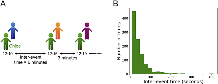
The waiting-time paradox applies to much more than just waiting for buses. Inter-event times are important in many situations. Consider the “event” of talking to a classmate at school. The inter-event times are the amounts of time between conversations with classmates (see Figure 3A). One inter-event time may be 2 minutes, and the next one may be 11 minutes. In social activities, unlike in bus schedules, there are often large variations in inter-event times. In Figure 3B, we show a histogram of inter-event times for a student in a school in France [3]. In the histogram, we list the times from left to right in increasing order. The height of each bar in the histogram indicates the number of times that each inter-event time occurs. Most inter-event times are short (such as 20 or 40 seconds), but a small number of them are large (such as between 200 and 400 seconds).
- Figure 3 - Inter-event times for a student socializing in a school.
- (A) The inter-event times for a student named Chloe. Chloe talks to three different students, with inter-event times of 6 minutes and 3 minutes. (B) A histogram of the inter-event times for a student in a school in France. This example comes from the “Primary School” data set in the SocioPatterns project [3]. We selected the student with the largest number of events and calculated all of that student’s inter-event times. The bars in this picture indicate the number of inter-event times of each duration for that student. The histogram shows that there are large variations in inter-event times. Most of them are short, but some of them are very long.
In our example of the waiting-time paradox with buses, we saw that even if there are only three long inter-event times among nine total inter-event times, we are more likely to get one of the long inter-event times than one of the short ones. This is an example of biased sampling. Another famous example of biased sampling is the friendship paradox [4, 5]. According to the friendship paradox, your friends tend to have more friends than you do. However, there is no reason to be upset, because this also is a purely mathematical phenomenon. If you have 20 friends in your school, many of them are likely to be popular people. For example, if Alice has just one friend, it is unlikely that you are Alice’s only friend; it is more likely to be someone else. By contrast, if Bob is friends with half of the students in your school, then it is very likely that you are one of Bob’s friends. Waiting for the next bus and counting the number of friends may seem to have nothing to do with each other. However, from a mathematical perspective, you are likely to have a friend like Bob for basically the same reason that you are likely to catch a bus after a long inter-event time. Suppose that there are six students who each have four friends and three students who each have 12 friends. If you are friends with just one of these 9 students, then your friend is likely to be a person with 12 friends, even though there are only three students with 12 friends among the 6 + 3 = 9 students. These numbers are exactly the same as the ones that we used in Figure 2 to demonstrate the waiting-time paradox. This illustrates that the waiting-time paradox and the friendship paradox have the same mathematical origin. Both are consequences of biased sampling.
An understanding of the waiting-time paradox is useful in many situations, such as for understanding how quickly a disease spreads in a population [6]. In university courses and scientific research, the waiting-time paradox shows up often in topics like probability theory, queuing theory, and network analysis. As we have seen, mathematics provides a way to unify seemingly different ideas and to see when they are closely related. This is true not just with the waiting-time paradox and the friendship paradox, but also with many other things.
Glossary
Waiting-Time Paradox: ↑ A mathematical phenomenon about times that seems like it may not make sense but is in fact correct. In the waiting-time paradox, if an event occurs at a time that we pick uniformly at random, the average waiting time until the next event is typically larger than half of the inter-event time. The waiting-time paradox is also called the “bus paradox” and the “inspection paradox.”
Inter-Event Time: ↑ The amount of time between two consecutive events, such as the arrivals of two buses at a bus stop or two conversations of a person with other people.
Probability Theory: ↑ A subject in mathematics about topics that are related to “probability,” which is a numerical description of how likely it is for an outcome to occur. A “probability distribution” is a mathematical function that gives the probabilities of all possible outcomes of something.
Uniformly at Random: ↑ A probability distribution in which each possible outcome is equally likely to occur.
Histogram: ↑ A diagram that shows the counts of items in several ranges of numbers to compare the count of the items in each range. For example, a histogram can show children with the age ranges 0–4 years, 5–9 years, 10–14 years, and so on. The height of the bar for the age range 10–14 years indicates the number of people who are between 10 and 14 years old.
Biased Sampling: ↑ Biased sampling occurs when one selects (or, to phrase it more technically, one “samples”) items, such as long inter-event times or a person with many friends, from a collection of items more often than other items as a result of the selection rules.
Conflict of Interest
The authors declare that the research was conducted in the absence of any commercial or financial relationships that could be construed as a potential conflict of interest.
Acknowledgments
We were grateful to our young readers—Nia Chiou, Taryn Chiou, Valerie E. Eng, Anthony Jin, Iris Leung, Maple Leung, Ami Masuda, and Ritvik Mukherjee—for their many helpful comments. We also thank their parents and teachers—Lyndie Chiou and Christina Chow—for putting us in touch with them and soliciting their feedback. We also thank Iris Leung for drawing Figure 1A. We thank our referee and editors for their helpful suggestions, and we thank the SocioPatterns collaboration (see http://www.sociopatterns.org) for providing data. NM acknowledges support from AFOSR European Office (grant number FA9550-19-1-7024). MAP acknowledges support from the National Science Foundation (grant number 1922952) through the Algorithms for Threat Detection (ATD) program.
References
[1] ↑ Welding, P. I. 1957. The instability of a close-interval service. J. Oper. Res. Soc. 8:133–42. doi: 10.1057/jors.1957.21
[2] ↑ Masuda, N., and Hiraoka, T. 2020. Waiting-time paradox in 1922. Northeast J. Complex Syst. 2:1. doi: 10.22191/nejcs/vol2/iss1/1
[3] ↑ Isella, L., Romano, M., Barrat, A., Cattuto, C., Colizza, V., Van den Broeck, W., et al. 2011. Close encounters in a pediatric ward: Measuring face-to-face proximity and mixing patterns with wearable sensors. PLoS ONE 6:e17144. doi: 10.1371/journal.pone.0017144
[4] ↑ Feld, S. L. 1991. Why your friends have more friends than you do. Am. J. Sociol. 96:1464–77. doi: 10.1086/229693
[5] ↑ Strogatz, S. 2012. Friends You Can Count On. The New York Times. Available online at: https://opinionator.blogs.nytimes.com/2012/09/17/friends-you-can-count-on/
[6] ↑ Karsai, M., Kivelä, M., Pan, R. K., Kaski, K., Kertész, J., Barabási, A. L. et al. 2011. Small but slow world: how network topology and burstiness slow down spreading. Phys. Rev. E 83:025102(R). doi: 10.1103/PhysRevE.83.025102